






商品详情
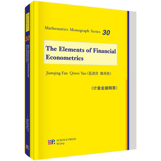
书名:计量金融精要
定价:198.0
ISBN:9787030433985
作者:范剑青
版次:1
出版时间:2026-07
内容提要:
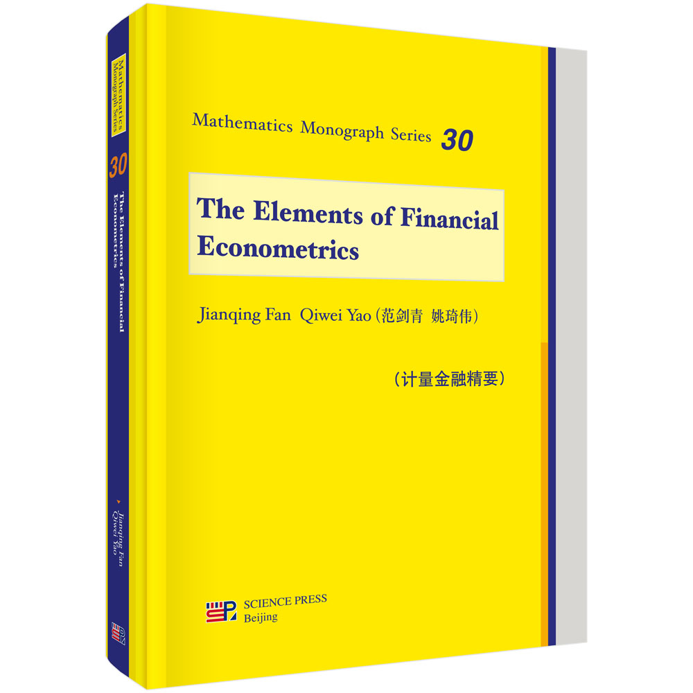
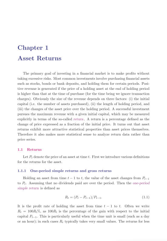
本书是一本关于金融计量方面的基础用书,提供了核心基础资料,包括金融研究日益增长的科学前沿和金融工业方面重要的发展情况。本书对资产定价理论、投资组合优化和风险管理方法提供了简洁的和紧凑的处理。提供了单因素和多因素情况下的时间序列模型技术,在分析财务数据上下文的时候介绍了他们的均值和方差。真实的数据分析贯穿全书,是本书的一个明显的特征。
目录:
Contents
Preface to Mathematics Monograph Series
Preface
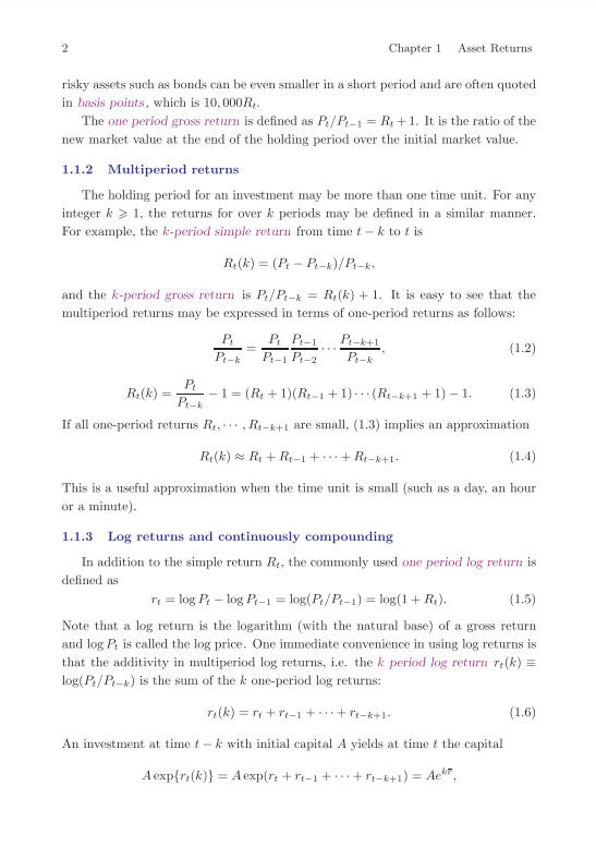
Chapter 1 Asset Returns 1
1.1 Returns 1
1.1.1 One-period simple returns and gross returns 1
1.1.2 Multiperiod returns 2
1.1.3 Log returns and continuously compounding 2
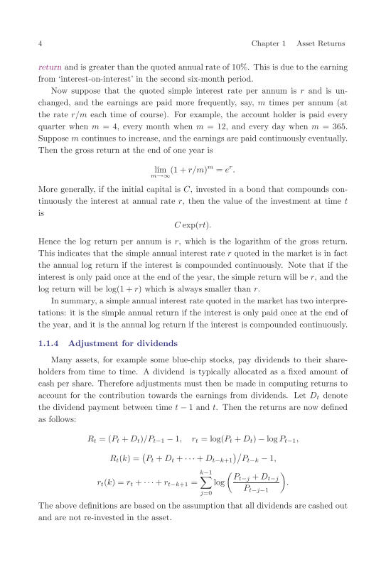
1.1.4 Adjustment for dividends 4
1.1.5 Bond yields and prices 5
1.1.6 Excess returns 6
1.2 Behavior of financial return data 7
1.2.1 Stylized features of financial returns 12
1.3 Efficient markets hypothesis and statistical models for returns 16
1.4 Tests related to efficient markets hypothesis 20
1.4.1 Tests for white noise 20
1.4.2 Remarks on the Ljung-Box test* 22
1.4.3 Tests for random walks 23
1.4.4 Ljung-Box test and Dickey-Fuller test 26
1.5 Appendix: Q-Q plot and Jarque-Bera test 26
1.5.1 Q-Q plot 26
1.5.2 Jarque-Bera test 27
1.6 Further reading and software implementation 28
1.7 Exercises 29
Chapter 2 Linear Time Series Models 31
2.1 Stationarity 31
2.2 Stationary ARMA models 33
2.2.1 Moving average processes 34
2.2.2 Autoregressive processes 38
2.2.3 Autoregressive and moving average processes 45
2.3 Nonstationary and long memory ARMA processes 50
2.3.1 Random walks 50
2.3.2 ARIMA model and exponential smoothing 52
2.3.3 FARIMA model and long memory processes* 53
2.3.4 Summary of time series models 54
2.4 Model selection using ACF, PACF and EACF* 55
2.5 Fitting ARMA models: MLE and LSE 59
2.5.1 Least squares estimation 59
2.5.2 Gaussian maximum likelihood estimation 61
2.5.3 Illustration with gold prices 63
2.5.4 A snapshot of maximum likelihood methods* 67
2.6 Model diagnostics: residual analysis 69
2.6.1 Residual plots 69
2.6.2 Goodness-of-fit tests for residuals 72
2.7 Model identification based on information criteria 73
2.8 Stochastic and deterministic trends 75
2.8.1 Trend removal 76
2.8.2 Augmented Dickey-Fuller test 77
2.8.3 An illustration 79
2.8.4 Seasonality 82
2.9 Forecasting 84
2.9.1 Forecasting ARMA processes 84
2.9.2 Forecasting trends and momentum of financial markets 89
2.10 Appendix: Time series analysis in R 97
2.10.1 Start up with R 97
2.10.2 R-functions for time series analysis 98
2.10.3 TSA – an add-on package 99
2.11 Exercises 100
Chapter 3 Heteroscedastic Volatility Models 104
3.1 ARCH and GARCH models 105
3.1.1 ARCH models 105
3.1.2 GARCH models 110
3.1.3 Stationarity of GARCH models 113
3.1.4 Fourth moments 115
3.1.5 Forecasting volatility 118
3.2 Estimation for GARCH models 120
3.2.1 Conditional maximum likelihood estimation 120
3.2.2 Model diagnostics 122
3.2.3 Applications of GARCH modeling 124
3.2.4 Asymptotic properties* 131
3.2.5 Least absolute deviations estimation* 132
3.3 ARMA-GARCH models 136
3.4 Extended GARCH models 137
3.4.1 EGARCH models 138
3.4.2 Asymmetric power GARCH 143
3.4.3 Excess returns and GARCH-in-Mean 146
3.4.4 Integrated GARCH model 147
3.5 Stochastic volatility models 148
3.5.1 Probabilistic properties 149
3.5.2 Parameter estimation 149
3.5.3 Leverage effects 152
3.6 Appendix: State space models* 153
3.6.1 Linear models 153
3.6.2 Kalman recursions for Gaussian models 153
3.6.3 Nonlinear models 156
3.6.4 Particle filters 158
3.7 Exercises 160
Chapter 4 Multivariate Time Series Analysis 163
4.1 Stationarity and auto-correlation matrices 163
4.1.1 Stationary vector processes 163
4.1.2 Sample cross-covariance/correlation matrices 165
4.2 Vector autoregressive models 168
4.2.1 Stationarity 169
4.2.2 Parameter estimation 170
4.2.3 Model selection and diagnostics 173
4.2.4 Illustration with real data 175
4.2.5 Granger causality 179
4.2.6 Impulse response functions 182
4.3 Cointegration 185
4.3.1 Unit roots and cointegration 186
4.3.2 Engle-Granger method and error correction models 187
4.3.3 Johansen’s likelihood method* 191
4.3.4 Illustration with real data 195
4.4 Exercises 199
Chapter 5 Efficient Portfolios and Capital Asset Pricing Model 201
5.1 Efficient portfolios 201
5.1.1 Returns and risks of portfolios 201
5.1.2 Portfolio optimization 202
5.1.3 Efficient portfolios and Sharpe ratios 205
5.1.4 Efficient frontiers 206
5.1.5 Challenges of implementation 207
5.2 Optimizing expected utility function 208
5.3 Capital asset pricing model 210
5.3.1 Market portfolio 210
5.3.2 Capital asset pricing model 212
5.3.3 Market β and its applications 214
5.4 Validating CAPM 215
5.4.1 Econometric formulation 215
5.4.2 Maximum likelihood estimation 216
5.4.3 Testing statistics 218
5.5 Empirical studies 223
5.5.1 An overview 223
5.5.2 Fama-French portfolios 224
5.5.3 Further remarks 227
5.6 Cross-sectional regression 227
5.7 Portfolio optimization without a risk-free asset 228
5.8 CAPM with unknowing risk free rate 236
5.8.1 Validating the Black version of CAPM 237
5.8.2 Testing statistics 237
5.9 Complements 240
5.9.1 Proof of (5.43) 240
5.9.2 Proof of (5.48) 240
5.10 Exercises 241
Chapter 6 Factor Pricing Models 245
6.1 Multifactor pricing models 245
6.1.1 Multifactor models 245
6.1.2 Factor pricing models 249
6.2 Applications of multifactor models 250
6.3 Model validation with tradable factors 251
6.3.1 Existence of a risk-free asset 252
6.3.2 Estimation of risk premia 252
6.3.3 Testing statistics 253
6.3.4 An empirical study using Fama-French portfolios 256
6.3.5 Absence of a risk-free asset* 258
6.4 Macroeconomic variables as factors* 260
6.5 Selection of factors 261
6.5.1 Principal component analysis 262
6.5.2 Factor analysis* 267
6.6 Exercises 269
Chapter 7 Portfolio Allocation and Risk Assessment 272
7.1 Risk assessment of large portfolios 272
7.1.1 Stability of a portfolio 273
7.1.2 Stability and risk approximations 274
7.1.3 Errors in risk assessments 279
7.1.4 Representative portfolios with a given exposure 281
7.2 Estimation of a large volatility matrix 282
7.2.1 Exponential smoothing 282
7.2.2 Regularization by thresholding 284
7.2.3 Projections onto semi-positive and positive definite matrix spaces 287
7.2.4 Regularization by penalized likelihood* 288
7.2.5 Factor model with observable factors 291
7.2.6 Approximate factor models with observable factors 295
7.2.7 Approximate factor models with unobservable factors 298
7.3 Portfolio allocation with gross-exposure constraints 301
7.3.1 Portfolio selection with gross-exposure constraint 302
7.3.2 Relation with covariance regularization* 305
7.4 Portfolio selection and tracking 306
7.4.1 Relation with regression 306
7.4.2 Portfolio selection and tracking 307
7.5 Empirical applications 308
7.5.1 Fama-French 100 portfolios 309
7.5.2 Russell 3000 stocks 311
7.6 Complements 312
7.6.1 Proof of Theorem 7.2 312
7.6.2 Proof of Theorem 7.3 313
7.6.3 Proof of (7.48) 313
7.7 Exercises 314
Chapter 8 Consumption based CAPM 316
8.1 Utility optimization 316
8.2 Consumption-based CAPM 319
8.2.1 CCAPM 319
8.2.2 Power utility 321
8.3 Mean-variance frontier* 325
8.4 Exercises 327
Chapter 9 Present-value Models 328
9.1 Fundamental price 328
9.2 Rational bubbles 330
9.3 Time-varying expected returns 332
9.4 Empirical evidence 336
9.5 Linear regression under dependence 344
9.6 Exercises 346
References 348
Author Index 358
Subject Index 362
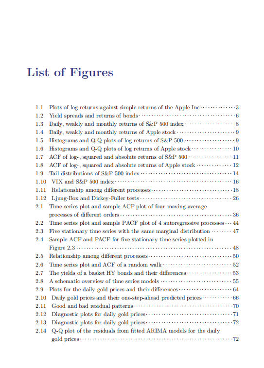
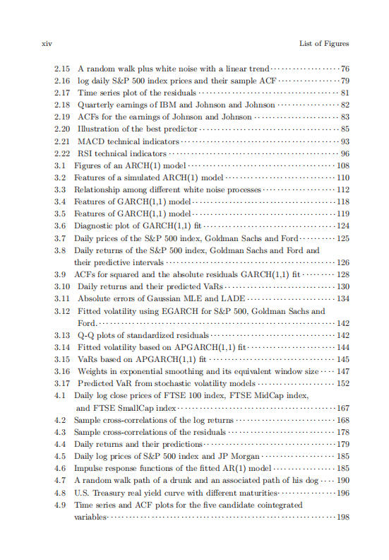
List of Figures
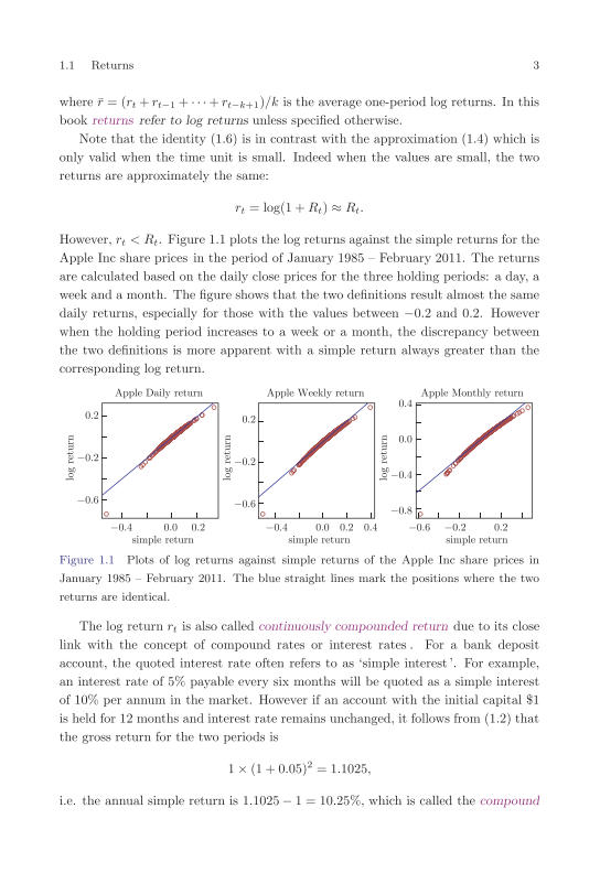
1.1 Plots of log returns against simple returns of the Apple Inc 3
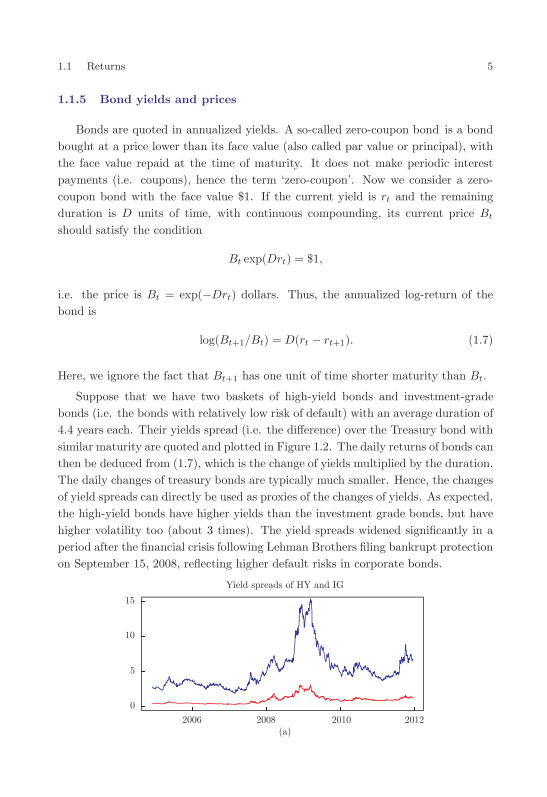
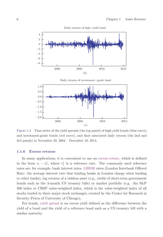
1.2 Yield spreads and returns of bonds 6
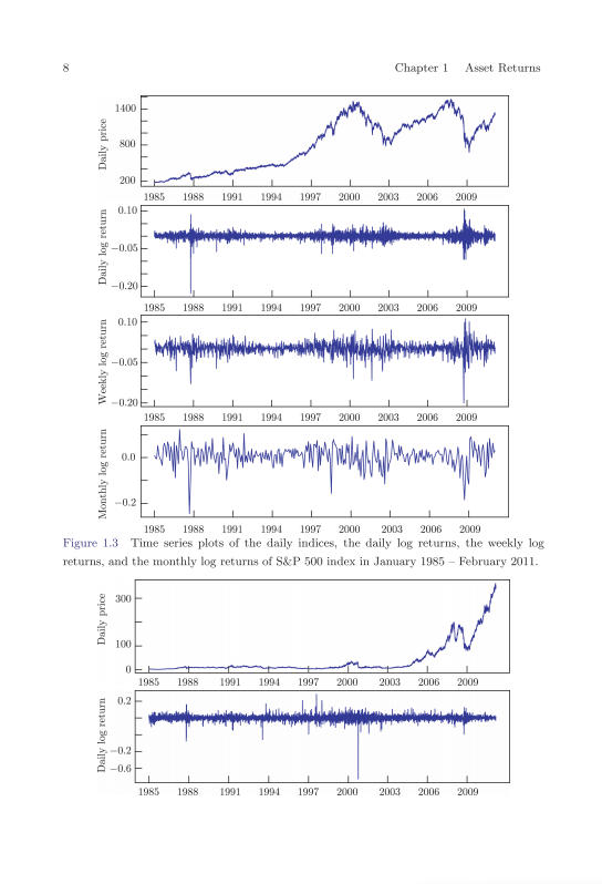
1.3 Daily, weakly and monthly returns of S&P 500 index 8
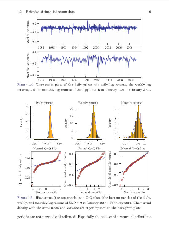
1.4 Daily, weakly and monthly returns of Apple stock 9
1.5 Histograms and Q-Q plots of log returns of S&P 500 9
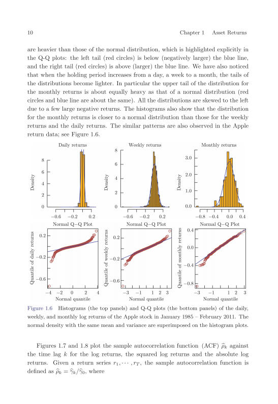
1.6 Histograms and Q-Q plots of log returns of Apple stock 10
1.7 ACF of log-, squared and absolute returns of S&P 500 11
1.8 ACF of log-, squared and absolute returns of Apple stock 12
1.9 Tail distributions of S&P 500 index 14
1.10 VIX and S&P 500 index 16
1.11 Relationship among different processes 18
1.12 Ljung-Box and Dickey-Fuller tests 26
2.1 Time series plot and sample ACF plot of four moving-average processes of different orders 36
2.2 Time series plot and sample PACF plot of 4 autoregressive processes 44
2.3 Five stationary time series with the same marginal distribution 47
2.4 Sample ACF and PACF for five stationary time series plotted in Figure 2.3 48
2.5 Relationship among different processes 50
2.6 Time series plot and ACF of a random walk 52
2.7 The yields of a basket HY bonds and their differences 53
2.8 A schematic overview of time series models 55
2.9 Plots for the daily gold prices and their differences 64
2.10 Daily gold prices and their one-step-ahead predicted prices 66
2.11 Good and bad residual patterns 70
2.12 Diagnostic plots for daily gold prices 71
2.13 Diagnostic plots for daily gold prices 72
2.14 Q-Q plot of the residuals from fitted ARIMA models for the daily gold prices 72
2.15 A random walk plus white noise with a linear trend 76
2.16 log daily S&P 500 index prices and their sample ACF 79
2.17 Time series plot of the residuals 81
2.18 Quarterly earnings of IBM and Johnson and Johnson 82
2.19 ACFs for the earnings of Johnson and Johnson 83
2.20 Illustration of the best predictor 85
2.21 MACD technical indicators 93
2.22 RSI technical indicators 96
3.1 Figures of an ARCH(1) model 108
3.2 Features of a simulated ARCH(1) model 110
3.3 Relationship among different white noise processes 112
3.4 Features of GARCH(1,1) model 118
3.5 Features of GARCH(1,1) model 119
3.6 Diagnostic plot of GARCH(1,1) fit 124
3.7 Daily prices of the S&P 500 index, Goldman Sachs and Ford 125
3.8 Daily returns of the S&P 500 index, Goldman Sachs and Ford and their predictive intervals 126
3.9 ACFs for squared and the absolute residuals GARCH(1,1) fit 128
3.10 Daily returns and their predicted VaRs 130
3.11 Absolute errors of Gaussian MLE and LADE 134
3.12 Fitted volatility using EGARCH for S&P 500, Goldman Sachs and Ford 142
3.13 Q-Q plots of standardized residuals 142
3.14 Fitted volatility based on APGARCH(1,1) fit 144
3.15 VaRs based on APGARCH(1,1) fit 145
3.16 Weights in exponential smoothing and its equivalent window size 147
3.17 Predicted VaR from stochastic volatility models 152
4.1 Daily log close prices of FTSE 100 index, FTSE MidCap index, and FTSE SmallCap index 167
4.2 Sample cross-correlations of the log returns 168
4.3 Sample cross-correlations of the residuals 178
4.4 Daily returns and their predictions 179
4.5 Daily log prices of S&P 500 index and JP Morgan 185
4.6 Impulse response functions of the fitted AR(1) model 185
4.7 A random walk path of a drunk and an associated path of his dog 190
4.8 U.S. Treasury real yield curve with different maturities 196
4.9 Time series and ACF plots for the five candidate cointegrated variables 198
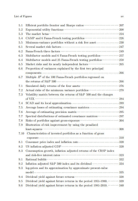
5.1 Efficient portfolio frontier and Sharpe ratios 207
5.2 Exponential utility functions 208
5.3 The market betas 210
5.4 CAMP and 6 Fama-French testing portfolios 224
5.5 Minimum-variance portfolios without a risk free asset 230
6.1 Several market risk factors 247
6.2 Fama-French three factors 249
6.3 Multifactor models and 6 Fama-French testing portfolios 257
6.4 Multifactor models and 25 Fama-French testing portfolios 258
6.5 Market risks and its nearly independent factors 265
6.6 Proportion of variances explained by the first two principal components 266
6.7 Multiple R2 of the 100 Fama-French portfolios regressed on the returns of S&P 500 266
7.1 Simulated daily returns of the four assets 276
7.2 Actual risks of the minimum variance portfolios 278
7.3 Volatility matrix between the returns of S&P 500 and the changes of VIX 284
7.4 SCAD and its local approximation 289
7.5 Average losses of estimating covariance matrices 294
7.6 Average of estimating precision matrix 295
7.7 Spectral distributions of estimated covariance matrices 297
7.8 Risks of portfolios against gross-exposure 304
7.9 Illustration of risk improvement by using the penalized least-squares 308
7.10 Characteristics of invested portfolios as a function of gross exposure 310
8.1 Consumer price index and inflation rate 320
8.2 US inflation adjusted GDP 320
8.3 Consumption growth, inflation adjusted returns of the CRSP index and risk-free interest rates 323
9.1 Rational bubble 332
9.2 Inflation adjusted S&P 500 index and its dividend 334
9.3 log-prices and its approximation by approximate present-value model 335
9.4 Dividend yield against future returns 338
9.5 Dividend yield against future returns in the period 1951-1980 339
9.6 Dividend yield against future returns in the period 1981-2010 340
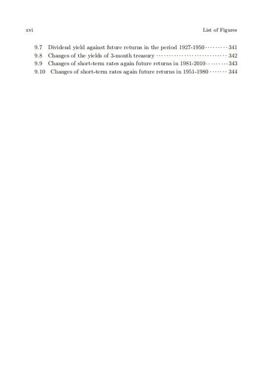
9.7 Dividend yield against future returns in the period 1927-1950 341
9.8 Changes of the yields of 3-month treasury 342
9.9 Changes of short-term rates again future returns in 1981-2010 343
9.10 Changes of short-term rates again future returns in 1951-1980 344 

- 科学出版社旗舰店 (微信公众号认证)
- 科学出版社秉承多年来形成的“高层次、高水平、高质量”和“严肃、严密、严格”的优良传统与作风,始终坚持为科技创新服务、为传播与普及科学知识服务、为科学家和广大读者服务的宗旨。
- 扫描二维码,访问我们的微信店铺
- 随时随地的购物、客服咨询、查询订单和物流...